The Network Has a Memory
Reconstructing what the network believed at 14:02, and the difference between what changed and what you learned
Michel Wijnberg
Every tool in this series so far answers questions about now. That is the wrong tense for the two moments an engineer most needs help.
The first is during an incident: the network is misbehaving, and what you need is not its current state but its state twenty minutes ago, before someone started fixing things. The second is after one: the network is fine again, everyone has a theory, and nobody can produce the topology as it stood when it broke.
Osprey’s answer is a clock.
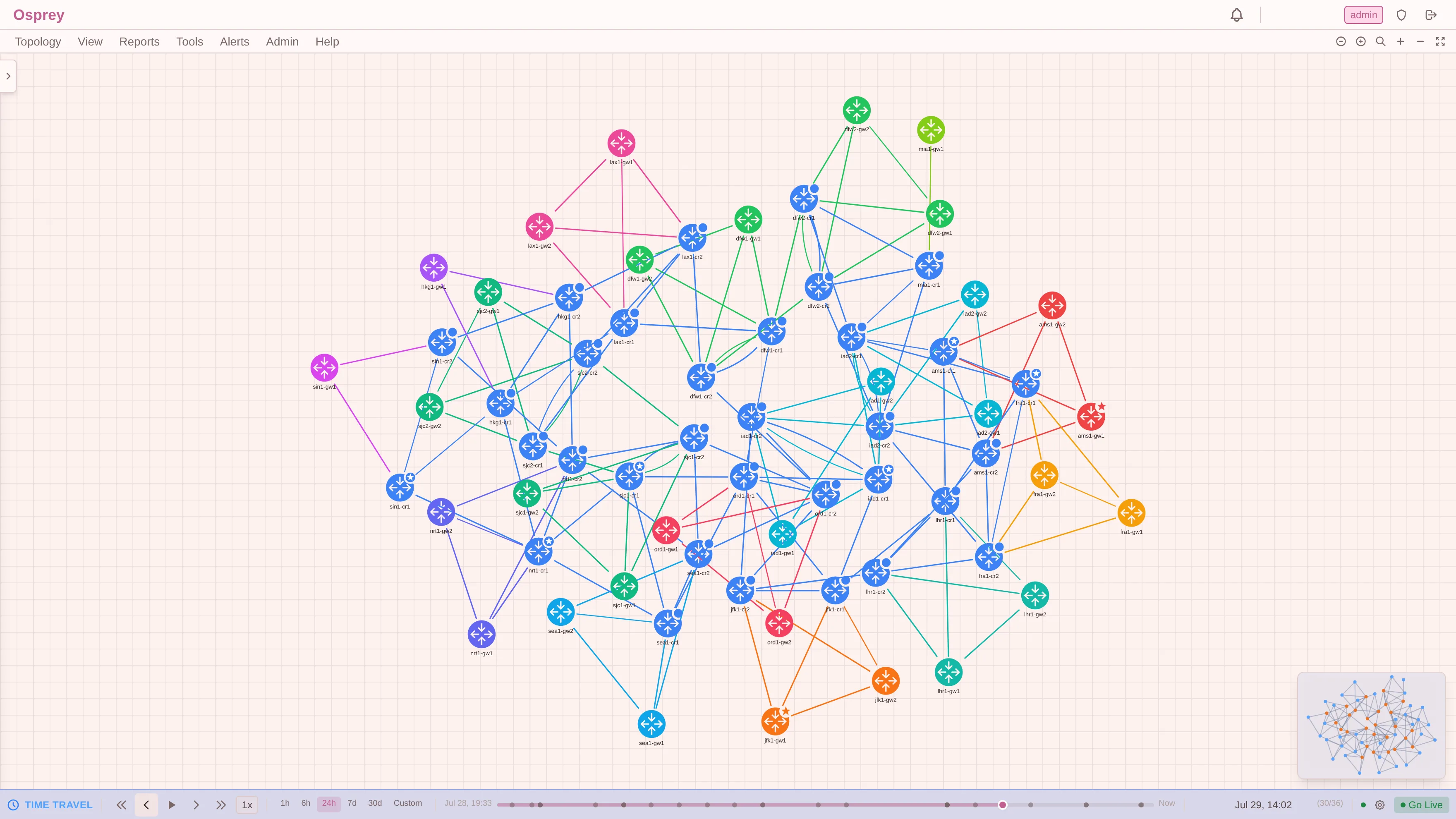
That is not a replay of a recording. Every element on that canvas was reconstructed
for a timestamp: the devices, the links, their costs and states, the area
memberships. The scrubber underneath says Jul 29, 14:02 and (30/36): the
thirtieth of thirty-six distinct topology states in the selected 24-hour window.
Each dot on that track is a moment the network was genuinely different.
Every monitoring tool keeps history, so that sentence needs a sharper edge. What they keep is measurements: CPU was 83%, the interface did 4 Gbit, the poll succeeded. Those are readings taken of the network, and at 14:02 they tell you a device was busy. They cannot tell you what it believed. What Osprey keeps is state: which adjacencies existed, which routes were installed and with what metric, which areas a router belonged to, which BGP paths were selected and why. The difference shows up the moment you ask a real question. A metrics history can tell you a link was saturated at 14:02. A state history can tell you the link was saturated because an ABR had withdrawn a summary four minutes earlier and half the region was suddenly taking the long way round. One is a symptom with a timestamp. The other is the network’s own reasoning, preserved.
Snapshots that only exist when something happened
The naive implementation writes a snapshot on a timer. Every five minutes, dump the topology. It is simple, and it produces a database mostly full of identical copies plus a resolution limit you cannot see past.
Osprey writes a snapshot when the topology changes, and never otherwise.
Every topology event from a collector is hashed first:
// computeTopologyHash computes an FNV-64a hash over the topology snapshot data.
// Uses addition accumulation of per-element hashes for order-independence.
Devices contribute their router ID and their ABR/ASBR bits, links contribute a direction-normalised router pair plus both costs and their state, stub networks and interfaces contribute theirs. Accumulation is additive so the hash does not depend on the order elements arrived in: two collectors reporting the same area in different sequence must produce the same hash, or every poll would look like a change.
The hash is compared against the last one for that area, in memory. Equal: nothing is written. Different: a snapshot row is inserted.
The result is a timeline that is information-dense by construction. Over the last 30 days my lab produced 478 snapshots across 51 areas: around 16 a day across the whole estate, each one an actual difference. The dots on the scrubber are not samples. They are events.
It also means a stable area can go many hours without a row, and that is correct rather than a gap: nothing happened, so there is nothing to record. The nearest snapshot at or before your chosen timestamp is the state at that timestamp.
Time travel is not one feature
The clock is the visible part. What makes it useful is that roughly twenty API
endpoints accept the same at= parameter and answer as of that moment: the topology
graph, the LSDB browser, path computation, SPF trees, per-router RIBs, inter-area and
external routes, ASBR entries, interfaces, stub networks, BGP peers, BGP best-paths,
per-peer received paths.
BGP gets a stronger treatment than snapshots, because BGP changes far more often than
topology. It is stored as a bitemporal changelog: every best-path, peer session
and (optionally) every received RIB entry is an interval with a valid_from and a
valid_to, where an open valid_to means “still true”. Asking a question as of T is
then a predicate rather than a reconstruction: valid_from <= T AND (valid_to IS NULL OR valid_to > T).
Two details in there are the ones that took the longest to get right, and both are about not recording things:
- Interval churn is suppressed by an attribute hash that deliberately excludes the IGP metric and resolved next-hop device. Those change whenever the IGP reconverges, and if they opened a new interval, every BGP prefix in the network would appear to flap each time an unrelated link cost moved.
- A peer going down is recorded as a monitoring gap, not as a mass withdrawal. When a BMP session drops, the router did not withdraw a hundred thousand prefixes. I simply stopped being told about them. Writing that as a withdrawal would manufacture the largest routing event in the history of the network, every time a monitoring session hiccuped.
Both are cases where the easy implementation invents an event. A history that invents events is worse than no history, because you will investigate them.
Simulating in the past
The two modes compose, and this is my favourite thing in the product.
You can enter time travel, position the clock, and then enter simulation. The
canvas carries a SIMULATION @ <timestamp> watermark, and the what-if runs against
the topology as it existed at that moment.
Which means the question you can ask is:
Would this failure have been survivable, given the network as it actually stood at 14:02?
Not against today’s topology, which has since been repaired, re-metriced and extended. Against the one that was really there. For post-incident work that is the difference between a defensible answer and a plausible one.
It honours its own limits, too. BGP peer-failure analysis at a past time requires full RIB history to have been recorded for that scope; where it was not, the result is not a silent approximation but a stated skip:
BGP effects (peer failure, hot-potato exit shifts, BGP traffic) are not evaluated at this time: no full-RIB history (history_mode=‘full’) is recorded for the scope. Enable full history mode on a BMP target to time-travel BGP.
That message names the missing input and the setting that would provide it. It is a message you can act on.
What is not in the past, said out loud
Several things genuinely have no history, and the endpoints that touch them say so rather than quietly serving live data dressed as historical data.
Ask the LSDB browser for a past moment and the response carries:
Topology and route LSAs reflect the selected time; LSA header metadata (age/seq/ checksum) is not historized and shows live values.
Ask for a cross-domain path at a past moment and, only where the answer actually leaned on live evidence, the explanation grows extra steps:
Time travel: L2 detail is live: L2/port annotations on this path reflect current LLDP/CDP wiring, not the selected time. L2 adjacency is not historized.
Time travel: entry resolved via current router-id: identity attributes (router-id, local address) are not historized and were borrowed from the live session record.
The conditionality matters. A stitch proven entirely from history carries neither note, so the notes mean something when they do appear. A blanket “some data may be live” disclaimer on every historical view would be technically true, permanently ignored, and useless.
There is one more limit I will state plainly because you would otherwise find it by being confused: link utilization colouring is switched off during time travel. The traffic heatmap goes blank rather than showing you live load on a historical topology. That is the safe behaviour and the wrong one. Blank reads as “no traffic” when it should read as “not available at this time”. The reader that would fix it is scheduled, not built.
The difference between what changed and what you learned
Time travel has a companion report: compare two moments and list the differences.
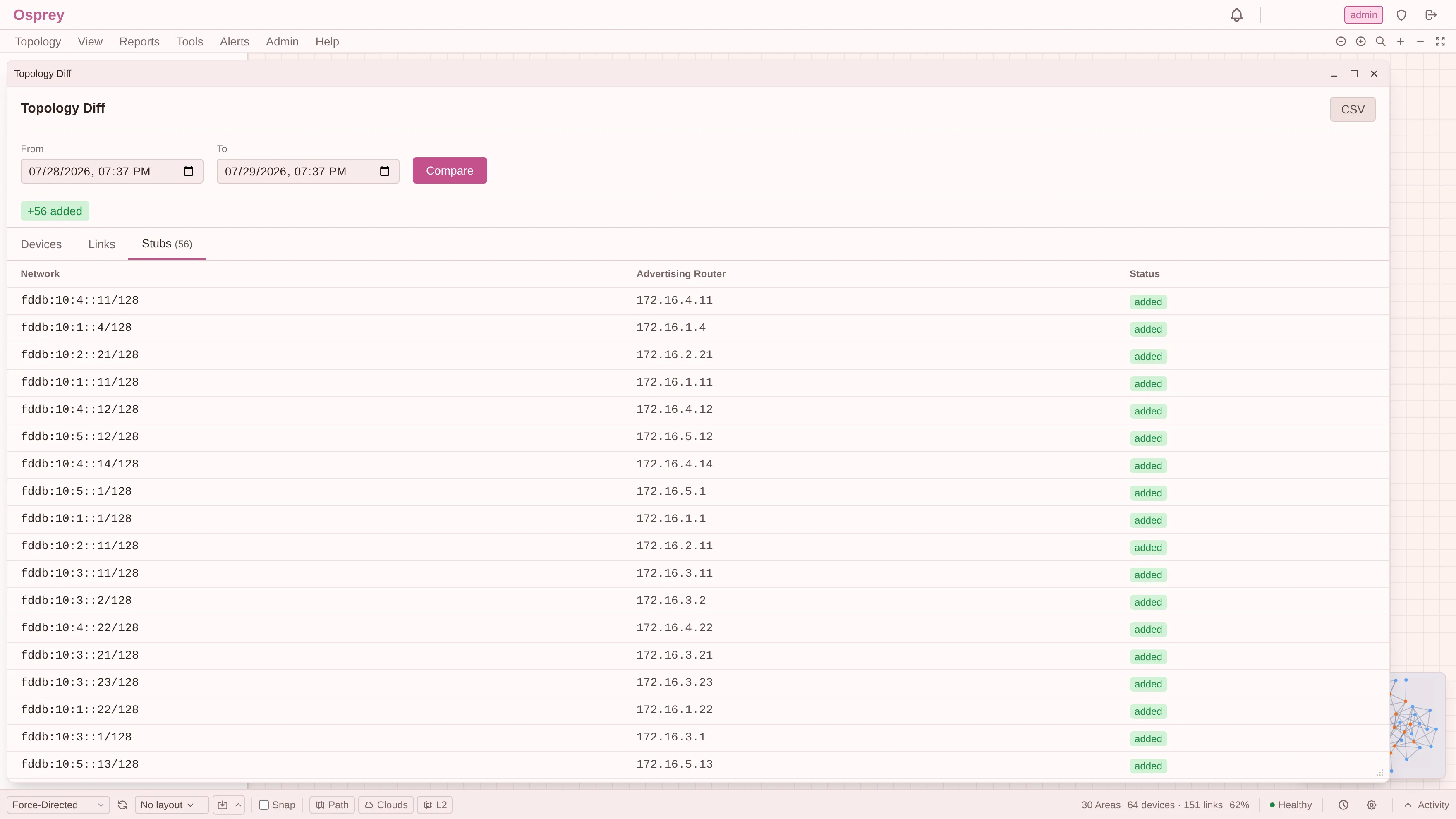
Over the last 24 hours in AS 200: no devices added, removed or changed. No links added
or removed. And 56 stub networks added, every one of them an IPv6 /128 loopback.
That looks like a network change. It is not one.
I checked when those 56 prefixes first entered the database, and every one of them
arrived between 10:00:49 and 10:01:14 this morning: a 25-second window. No
network reconfigures 56 loopbacks across 64 routers in 25 seconds. What happened was a
discovery pass: those prefixes had been in the OSPFv3 database all along, and this is
the moment Osprey started recording them.
This distinction deserves a name, because conflating the two sends people hunting for a change that never happened:
A topology diff tells you what the model learned. It is not the same thing as what the network did.
Sometimes they coincide: a link goes down, the model records a link going down. Sometimes they do not, and the giveaway is usually the shape of the timestamps: real network changes arrive with the timing of protocol convergence, and model changes arrive with the timing of a poll cycle. Fifty-six identical prefixes in 25 seconds is a poll cycle wearing a change’s clothing.
An observability product that cannot tell you which of the two you are looking at will eventually cost someone an afternoon. Osprey does not label it automatically. The diff shows what the model recorded, and the reasoning above is mine, not the tool’s. But every row carries the timestamps you need to make the call yourself, which is the minimum I think honest tooling owes you.
Where this series ends
Three series, and really one argument, arrived at from three directions.
Series 1 was about whether the model is true: model the network as it actually is, observe it without becoming part of it, reproduce forwarding hop by hop, and refuse to guess.
Series 2 was about whether the evidence is rankable: hold several truths at once, grade contradictory sources, find your own mistakes before your customers do.
Series 3 was about what that buys you: a model correct enough to reason with. Break something and see what happens. Ask what depends on what. Estimate what you cannot measure, and say that you are estimating. Ask what the network believed an hour before it broke.
None of that works on a model you do not trust. Every honest refusal in Series 1 and every graded piece of evidence in Series 2 exists so that the answers in Series 3 mean something: a what-if built on a topology that is 9% fiction is not a planning tool, it is a random number generator with a nice canvas.
Post eight gave that argument its shortest form: a topology engine is a compiler for network state: messy, contradictory input, a deterministic model out, and the routers themselves as the oracle. Compilers are judged by conformance rather than plausibility, and every refusal in these twelve posts is what conformance costs on the cases where the answer is not available.
Get the model right. Say how you know. Then, and only then, start asking it questions.
The full series: Trust: Three IGPs, One Map · Zero Footprint · Hop-by-Hop Truth · What Osprey Refuses to Guess. Engineering the Truth: The Same Router, Three Different Truths · When the Network Disagrees With Itself · The Day My Topology Lied to Me · A Network Engineer’s Unit Tests. From Seeing to Reasoning: What Happens If I Break This? · The Blast Radius · Estimating What You Cannot Measure · this one.