The Same Router, Three Different Truths

The first four posts in this series were about trust: model the network correctly, observe it safely, reproduce forwarding honestly, and refuse to guess. This one starts a second set, about what it actually takes to hold that line.

And it starts with the thing that breaks most topology tools before they get anywhere near an interesting question: a router is not one thing.

---

A router with two of everything

Here is nrt1-cr1 from my lab:

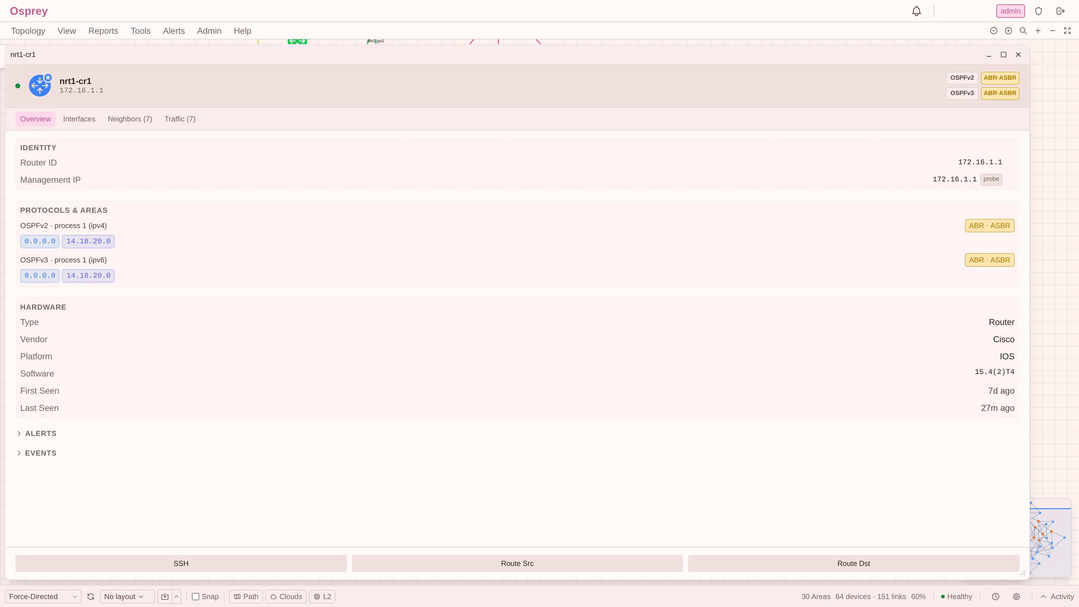
Look at the top right. Not one role badge. Two:

OSPFv2   ABR·ASBR
OSPFv3   ABR·ASBR

And underneath, in Protocols & Areas:

Protocol instance	Areas	Role
OSPFv2 · process 1 (ipv4)	0.0.0.0, 14.18.20.0	ABR · ASBR
OSPFv3 · process 1 (ipv6)	0.0.0.0, 14.18.20.0	ABR · ASBR

It looks like duplication. It isn’t. These are two independent protocol instances with two independent link-state databases, and nrt1-cr1 earns the ABR title separately in each by being attached to more than one area in that instance. The area labels match because someone numbered them to match, not because they are the same object. In the database they have different UUIDs, because OSPFv2 area 14.18.20.0 and OSPFv3 area 14.18.20.0 are different areas that happen to share a name.

That distinction sounds pedantic right up until the two disagree. Which, as it turns out, they always do.

---

One wire, two costs, one hundred percent of the time

Here is a single physical link between two routers:

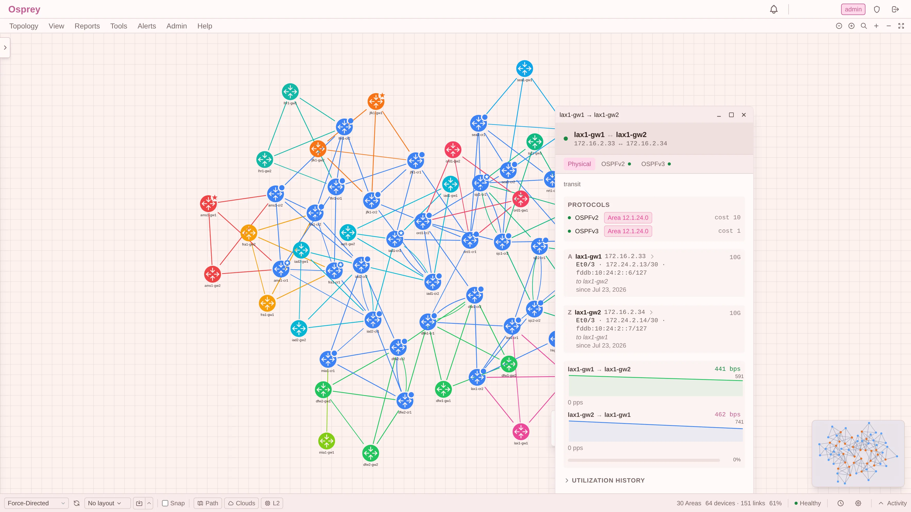
One cable. Et0/3 to Et0/3, 10G, carrying 172.24.2.13/30 and fddb:10:24:2::6/127. Osprey draws it as one edge, because physically it is one edge, and gives it a tab per protocol.

Now read the costs:

OSPFv2   Area 12.1.24.0   cost 10
OSPFv3   Area 12.1.24.0   cost 1

Same wire. Same area number. Different metric.

I did not stage that for the screenshot. I checked every dual-stack link in AS 200 afterwards, and the result is more interesting than the single example:

Dual-stack links in AS 200	124
…where OSPFv2 and OSPFv3 costs differ	124 (100%)
at (v2 = 10, v3 = 1)	85
at (v2 = 10000, v3 = 10)	39

Every single one differs, but look at the two groups: 39 links are a factor 1000 apart, and 85 are a factor 10 apart. That asymmetry is the interesting part, and it took asking the router to explain it.

Routing Process "ospf 1"     Reference bandwidth unit is 100000 mbps
Routing Process "ospfv3 1"   Reference bandwidth unit is 100 mbps

One setting, not two. Cost is reference bandwidth divided by interface bandwidth, so both processes are scaling the same wires by numbers that differ by exactly 1000. On the 10 Mbps links that arrives intact: 10000 against 10. On the 10 Gbps links OSPFv3 computes 100/10000 = 0.01, and the minimum cost a router will advertise is 1. The floor eats the rest.

So the distortion is not uniform, and that is precisely what makes it dangerous. A uniform scaling would be harmless: multiply every cost in a topology by the same constant and the shortest path does not move. Here the constant is 1000 on some links and 10 on others, because a clamp intervened. The two protocols therefore rank the same links differently against each other, and IPv4 and IPv6 traffic can take different paths across this network. You cannot eyeball which ones. You have to compute both.

A tool that renders “one link, one cost” has to pick one of those two numbers. Whichever it picks, it is wrong half the time, and it will never tell you which half you are in.

---

Why the hierarchy is load-bearing

This is the reason Osprey’s data model is not Node, Edge, Protocol:

Network → Autonomous System → Routing Domain → Protocol Instance → Area → Device
                                                                      ↳ Interface

Each level exists because something in the network can differ across it:

• Network: the tenant boundary. The same physical box can be monitored under two tenants with different credentials and different views.
• Autonomous System: the BGP identity, and the scope a BMP feed belongs to.
• Routing Domain: global table, a VRF, or an L3VPN. Same router, different routing tables, genuinely different reachability.
• Protocol Instance: unique on (routing domain, protocol, process id, address family). This is the level that makes nrt1-cr1 two routers.
• Area: where the LSDB actually lives, and therefore where SPF actually runs.
• Device: many-to-many with areas, via a membership table. Not a foreign key. A foreign key would have forced the lie that a router lives in one area.

And interfaces are scoped by (device_id, if_index, area_id), because the same physical port participates in several protocol instances at once, with a different cost, a different neighbour state and a different address family in each.

Derived roles fall out of that structure instead of being stored as labels:

• ABR = attached to more than one area within an instance
• ASBR = the E-bit set in the router’s own LSA (RFC 2328 §A.4.2), which is the router stating that it originates external routing information. Not a membership count: a router can be an ASBR while living in a single area, and it can span several instances without being one
• VRF-Lite = present in more than one routing domain

Which is why nrt1-cr1 can be an ABR twice, and why the badge is drawn twice. Nobody typed “ABR” anywhere. It is a consequence of the memberships, recomputed from the LSDBs.

---

The topologies are all real at once

The useful way to think about this is that there is no such thing as the topology. There are several, they are all simultaneously true, and they answer different questions:

Topology	Built from	Answers
Physical	LLDP / CDP, IP-MIB	What is cabled to what
L2	Bridge/VLAN adjacency	What shares a broadcast domain
IGP (per instance)	LSDB per protocol per area	What each protocol believes
BGP	BMP RIB	What is reachable and via whom
Forwarding	Each router’s own table	Where a packet actually goes

“Are A and B connected?” has five different correct answers depending on which of those you meant. Two routers can share a cable and no IGP adjacency. They can share an IGP adjacency and never forward a packet to each other. They can be BGP peers over a path that crosses three boxes neither of them can see.

Post three was really an argument about the last two rows: that the IGP topology and the forwarding topology are not the same graph, and treating them as one produced fictional paths one time in eight. This post is the same argument one level down: the physical topology and the protocol topology are not the same graph either, and 124 links in my lab prove it with a factor of ten.

---

What this costs

Being honest about this is not free. It means:

• Two LSDBs to walk where a simpler tool walks one
• A membership table instead of a foreign key
• Roles recomputed rather than stored
• Every path query needing to know which instance and which address family it is being asked about
• A UI that has to show a tab strip on a link instead of a number

The alternative is a graph that renders faster, demos better, and quietly picks one of two costs on every dual-stack link in your network.

I have run networks where the IPv4 and IPv6 paths diverged and nobody noticed for months, because every tool on the wall drew one line between two routers. The line was not wrong. It was just answering a question nobody had asked.

---

Next: what happens when those sources contradict each other outright: When the Network Disagrees With Itself.